Diagnostics Overview

This diagnostics package is part of the CADRE EPIC FV3-JEDI training workflow and is used in the 2026 CADRE Data Assimilation Workshop (https://epic.noaa.gov/cadre-epic-data-assimilation-training/). The tools support the hands-on sessions for the FV3-JEDI hybrid 3D-Var canned case (C96/C48), providing participants with a unified framework for analyzing background fields, increments, observation departures, spectral characteristics, and chi-squared consistency. The same diagnostics are used throughout the CADRE Year 2 experiments, including the ATMS, GNSSRO, ASCAT, and surface pressure components of the FV3-JEDI system.

The diagnostics toolkit provides a unified set of tools for analyzing background fields, increments, observation departures, and spectral properties of the data assimilation system. In addition to the standard diagnostic capabilities—increment maps, zonal means, observation histograms, satellite scan‑position bias checks, and latitude‑binned statistics—the toolkit includes two advanced diagnostic components:

1. Power Spectral Analysis Used to quantify how variance is distributed across spatial scales and how experiments (e.g., NICAS length‑scale changes) modify the spectral characteristics of increments and background fields.

2. Extended RMS Statistics Channel‑wise diagnostics of O–B and O–A bias, RMS, normalized RMS, bias‑corrected RMS, and analysis improvement metrics. These extended statistics provide a detailed view of observation‑space performance beyond simple mean and RMS values.

In addition, the toolkit supports a chi‑squared consistency check through automated parsing of JEDI log files. This diagnostic evaluates whether the ratio \(\mathrm{Jo}/p\) approaches unity, indicating consistency between observation errors, background errors, and the resulting analysis increments.

The following sections describe the mathematical formulation of these diagnostics and provide example figures illustrating their use.

Spectral Diagnostics

Overview

Spectral diagnostics quantify how variance is distributed across spatial scales. The UFS DA diagnostics compute isotropic 1‑D spectra derived from a full 2‑D horizontal Fourier transform. This reveals how the background (BKG), increments (INC), and experiment differences modify energy across scales.

2‑D Fourier Transform

For a horizontal field \(f(x, y)\) on an \(N_x \times N_y\) grid, the 2‑D Discrete Fourier Transform is

\[F(k_x, k_y) = \sum_{x=0}^{N_x-1} \sum_{y=0}^{N_y-1} f(x, y)\, e^{-i 2\pi \left( \frac{k_x x}{N_x} + \frac{k_y y}{N_y} \right)}\]

Each pair \((k_x, k_y)\) corresponds to one grid‑scale sinusoidal wave with a specific wavelength and direction.

Power Spectrum

The 2‑D power spectrum is

\[P(k_x, k_y) = |F(k_x, k_y)|^2\]

This represents the energy contribution of each grid‑scale wave.

Isotropic Spectrum

The 2‑D spectrum is radially averaged into bins of total wavenumber

\[K = \sqrt{k_x^2 + k_y^2}\]

to produce a 1‑D isotropic spectrum \(P(K)\). This gives the distribution of variance across spatial scales.

Parseval Consistency

The total variance in physical space equals the total power in spectral space:

\[\sum_{x,y} f(x,y)^2 = \frac{1}{N_x N_y} \sum_{k_x,k_y} |F(k_x, k_y)|^2\]

This ensures that the isotropic spectrum is a true variance decomposition by scale.

Background vs Increment Spectra (Control Experiment)

The background (BKG) spectrum typically follows a smooth power‑law decay, reflecting the model’s natural distribution of variance. The increment (INC) spectrum is much smaller and shows how the analysis updates redistribute variance across scales.

A healthy DA system produces increments that:

• contain most of their energy at large scales

• have very little high‑wavenumber energy

• do not inject noise at small scales

In the control experiment, the increment spectrum exhibits a large‑scale plateau. This is expected: the largest scales are dominated by broad, domain‑wide adjustments, and the isotropic bins at the smallest wavenumbers contain only a few modes, producing a flat appearance.

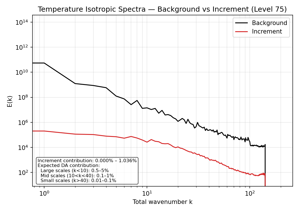
Background and increment spectra for temperature at model level 75 in the control experiment. The increment spectrum is smooth and confined to large scales. The plateau at the lowest wavenumbers reflects broad, domain‑scale adjustments and the small number of modes in the first isotropic bins.

Spectral Ratio (EXP vs CTRL)

The spectral ratio compares the scale‑dependent variance between two experiments:

\[R(K) = \frac{P_{\mathrm{EXP}}(K)}{P_{\mathrm{CTRL}}(K)}\]

Interpretation:

• \(R(K) > 1\) — EXP has more energy in the grid‑scale waves at scale \(K\)

• \(R(K) < 1\) — EXP has less energy at that scale

NICAS Length‑Scale Experiment

Increasing the NICAS horizontal correlation length scale broadens the static covariance’s spatial correlations. The static covariance itself is unchanged in shape; only the length scale parameter increases. This produces smoother increments and enhances variance at the largest spatial scales (small K), while reducing variance at smaller scales.

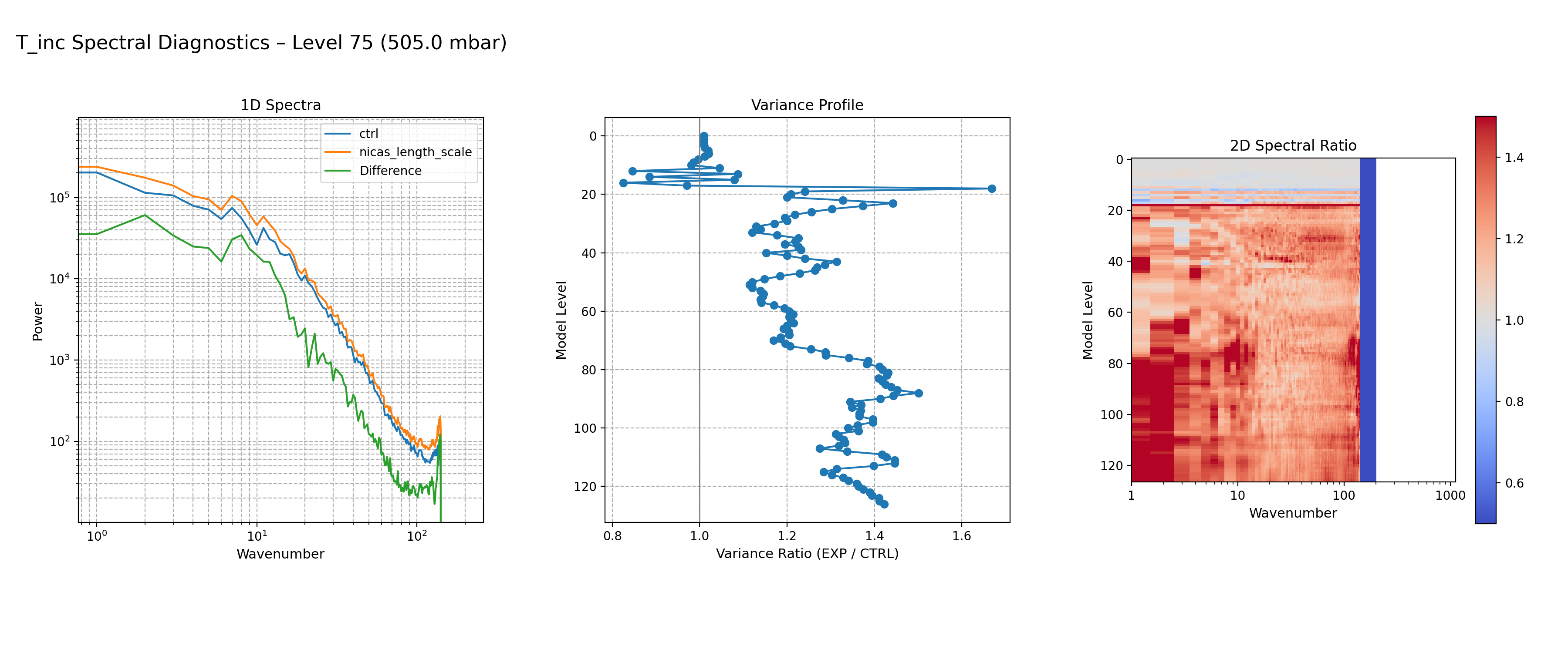
CTRL vs NICAS length‑scale increment spectra at model level 75. Increasing the NICAS horizontal correlation length scale boosts large‑scale variance and suppresses small‑scale variance, producing smoother increments.

Static Background Covariance Weight Experiment

This experiment increases the weight of the climatology‑based static background‑error covariance in the hybrid formulation. The static covariance itself is unchanged; only its relative contribution to the total hybrid covariance increases compared to the flow‑dependent ensemble covariance.

Increasing the static weight enhances variance at the largest spatial scales (small K) while suppressing variance at smaller scales. This produces smoother increments dominated by broad, domain‑scale structure.

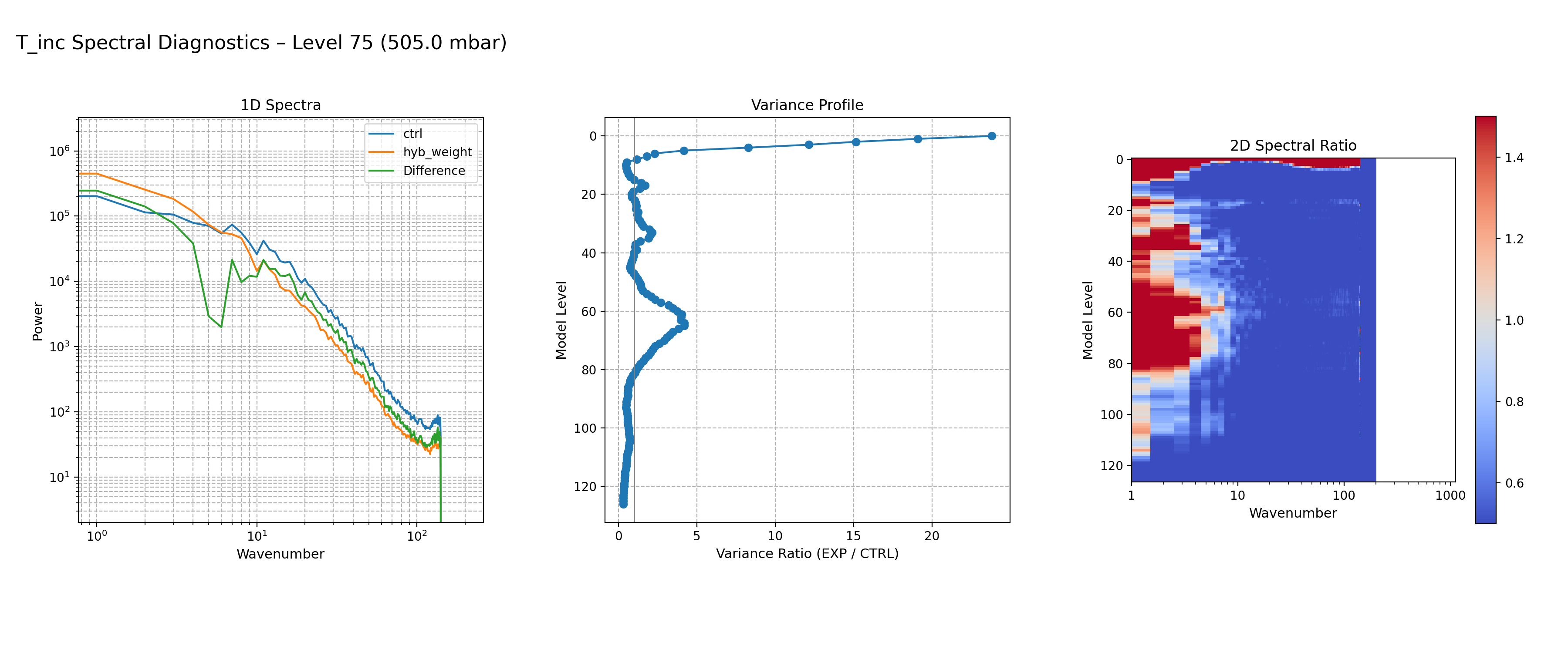
CTRL vs increased static background‑covariance weight for temperature increments at level 75. The increased static weight boosts large‑scale variance and damps small‑scale variance, reflecting the dominance of smoother climatological static covariance.

Observation Statistics

Formulation

Let \(y_i\) be an observation, and let \(H(x_b)_i\) and \(H(x_a)_i\) denote the background and analysis model equivalents. Define the departures:

\[d_{b,i} = y_i - H(x_b)_i, \qquad d_{a,i} = y_i - H(x_a)_i.\]

Mean (Bias)

\[\mu(d) = \frac{1}{N} \sum_{i=1}^{N} d_i\]

Meaning: Measures systematic error. A reduction from O–B to O–A indicates improved bias characteristics.

RMS (Root‑Mean‑Square Error)

\[\mathrm{RMS}(d) = \sqrt{\frac{1}{N} \sum_{i=1}^{N} d_i^2}\]

Meaning: Measures total error magnitude (bias + random error).

RMS Difference (Analysis Improvement)

\[\Delta \mathrm{RMS} = \mathrm{RMS}(d_a) - \mathrm{RMS}(d_b)\]

or normalized:

\[\Delta \mathrm{RMS}_{\text{rel}} = \frac{\mathrm{RMS}(d_a) - \mathrm{RMS}(d_b)}{\mathrm{RMS}(d_b)}\]

Meaning: Negative values indicate analysis improvement.

Normalized RMS

If observation error standard deviations \(\sigma_{o,i}\) are available:

\[d_{n,i} = \frac{d_i}{\sigma_{o,i}}, \qquad \mathrm{RMS}_n = \sqrt{\frac{1}{N} \sum_{i=1}^{N} d_{n,i}^2}\]

Meaning: - \(\mathrm{RMS}_n \approx 1\) → observation errors well specified - \(\mathrm{RMS}_n \gg 1\) → errors underestimated - \(\mathrm{RMS}_n \ll 1\) → errors overestimated

Bias‑Corrected RMS

\[\mathrm{BC\text{-}RMS}(d) = \sqrt{\frac{1}{N} \sum_{i=1}^{N} (d_i - \mu(d))^2}\]

Meaning: Measures random error only (bias removed).

Extended ATMS Statistics

Extended ATMS observation‑space diagnostics showing O–B and O–A bias, RMS, normalized RMS, bias‑corrected RMS, and analysis improvement metrics. These statistics quantify systematic error, total error, random error, and the degree to which the analysis reduces observation‑space departures.

Chi‑Square Consistency Check

The chi‑square consistency diagnostic evaluates whether the innovations (OMB) are broadly compatible with the assumed observation‑error variances. It provides a quick indication of whether the specified observation‑error model is reasonable.

For each observation i, the innovation d_b is scaled by its assumed observation‑error variance σ_{o,i}². The normalized innovation is

\[z_i = \frac{d_{b,i}}{\sigma_{o,i}}.\]

If the observation‑error model is reasonable, the average value of z_i² should be close to one. This leads to the chi‑square consistency measure

\[\chi^2 = \frac{1}{N} \sum_{i=1}^{N} \frac{d_{b,i}^2}{\sigma_{o,i}^2}.\]

Interpretation

• χ² ≈ 1 → observation‑error variances are broadly consistent with the size of

  the innovations.

• χ² >> 1 → observation‑error variances are likely too small (innovations too

  large).

• χ² << 1 → observation‑error variances are likely too large (innovations too

  small).

Practical Computation in JEDI

The toolkit computes this diagnostic by reading the JEDI log and using the reported values of Jo and the number of assimilated observations p:

\[\chi^2 \approx \frac{J_o}{p}.\]

Here Jo/p is a practical, heuristic average of the normalized innovation variance. It is not a formal statistical test, but it provides a quick sense of whether the assumed observation‑error variances are in a reasonable range.

Channel‑Wise Normalized RMS²

The obs_diagnostic.py (ufsda-obs-diag) script also computes a channel‑by‑channel normalized RMS² value for instruments such as ATMS:

\[\mathrm{NRMS}^2_c = \frac{1}{N_c} \sum_{i \in c} \frac{d_{b,i}^2}{\sigma_{o,i}^2},\]

where N_c is the number of assimilated observations in channel c.

This quantity is directly comparable to Jo/p, but computed separately for each channel rather than over all observations. Channel‑wise NRMS² helps identify channels with mis-specified observation errors or representativeness issues.

Reference

• Talagrand, O. (2003). Evaluation of probabilistic prediction systems. ECMWF Workshop on Diagnostics for Data Assimilation Systems.

Weather Events Diagnostics

The weather‑events module provides global synoptic‑scale diagnostics derived from FV3 ATM background fields. It identifies dynamically coherent features such as:

• 500 hPa cyclone centers (vorticity‑based)

• 250 hPa jet streaks (ridge detection)

• 850 hPa baroclinic zones (temperature‑gradient magnitude)

These diagnostics complement increment‑based tools by providing a large‑scale flow context for DA experiments.

See Weather Events Diagnostics for usage examples.